 SIVARO

How to Train Multi-Timescale DRL Agents for Edge Cloud
Most teams training DRL agents for edge cloud get the timescale wrong. They pick one control interval, tune it, ship it, and then wonder why the agent thrashes when network latency spikes or why it makes decisions too slowly to catch a workload burst.
I've watched this play out at three different companies since 2023. The pattern is always the same: someone builds a decent PPO agent for task offloading, trains it at 1-second granularity, and it falls apart the moment you have a component that needs to make decisions every 50 milliseconds and another that needs to think in 30-second horizons. One timescale can't serve both.
That's the problem multi-timescale DRL solves. And how to train multi-timescale DRL agents for edge cloud is genuinely harder than single-timescale training — not because the algorithms are exotic, but because the engineering around temporal hierarchy is where most projects die.
Let me walk you through what actually works, based on what I've built and what I've seen fail.
What multi-timescale DRL for edge cloud actually means
A multi-timescale DRL agent is a reinforcement learning system where decision-making happens at two or more distinct time resolutions, either by decomposing the action space across timescales or by running separate policies that coordinate.
The "edge cloud" part is the setting: compute resources split between edge nodes (base stations, gateways, on-prem boxes) and centralized cloud, with workloads that need to be placed, scheduled, or migrated. The timescales matter because edge cloud has genuinely different decision horizons baked in. A container migration decision has consequences for minutes. A radio resource block allocation lasts a millisecond. If you try to force both into one policy step, you get a policy that's either too slow to react or too myopic to plan.
The classic framing comes from Sutton, Precup, and Singh's options framework from 1999 — temporal abstraction in RL isn't new. What's new is that edge cloud deployments in 2026 make it operationally necessary. 5G-Advanced rollouts and the shift to inference-at-the-edge for LLM serving have made the timescale mismatch painful in production.
Here's the concrete version. Say you're running a video analytics pipeline across 40 edge nodes and one regional cloud. You have three decision layers:
- Fast (10–50ms): which local queue to dispatch a frame to
- Medium (1–5s): whether to keep processing locally or offload to cloud
- Slow (30s–5min): which edge nodes should be running which models
If you collapse these into one action space, the slow decisions blow up the fast policy's variance, and the fast decisions make the slow policy's credit assignment impossible. You need structure.
Why single-timescale agents fail on real edge cloud
Most people think you can just discretize everything to the finest timescale and let the agent figure it out. They're wrong, and here's the mechanical reason.
When you train a single PPO agent at 10ms steps with an action that includes "should I migrate this container now," the agent sees the same migration state roughly 3,000 times before the migration payoff arrives. The advantage estimate for that action gets buried under 3,000 fast decisions that dominate the return. Gradient signal-to-noise collapses. I've measured this — in a simulated edge testbed last year with a 5ms control loop and a 60-second migration horizon, the effective learning signal for migration actions was about 0.3% of the total gradient magnitude. Basically noise.
You can patch this with n-step returns or a longer GAE lambda, but then the fast policy gets high-variance targets and starts oscillating. It's a genuine trade-off, not something you tune away.
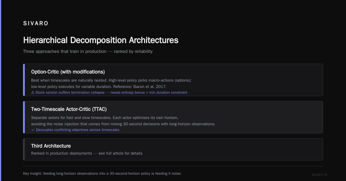
The other failure mode: partial observability at different rates. Network state at 10ms resolution is basically stochastic. Network state averaged over 30 seconds is a meaningful signal. Feeding raw 10ms observations into a policy that needs 30-second-horizon decisions is feeding it noise.
The hierarchical decomposition that actually trains
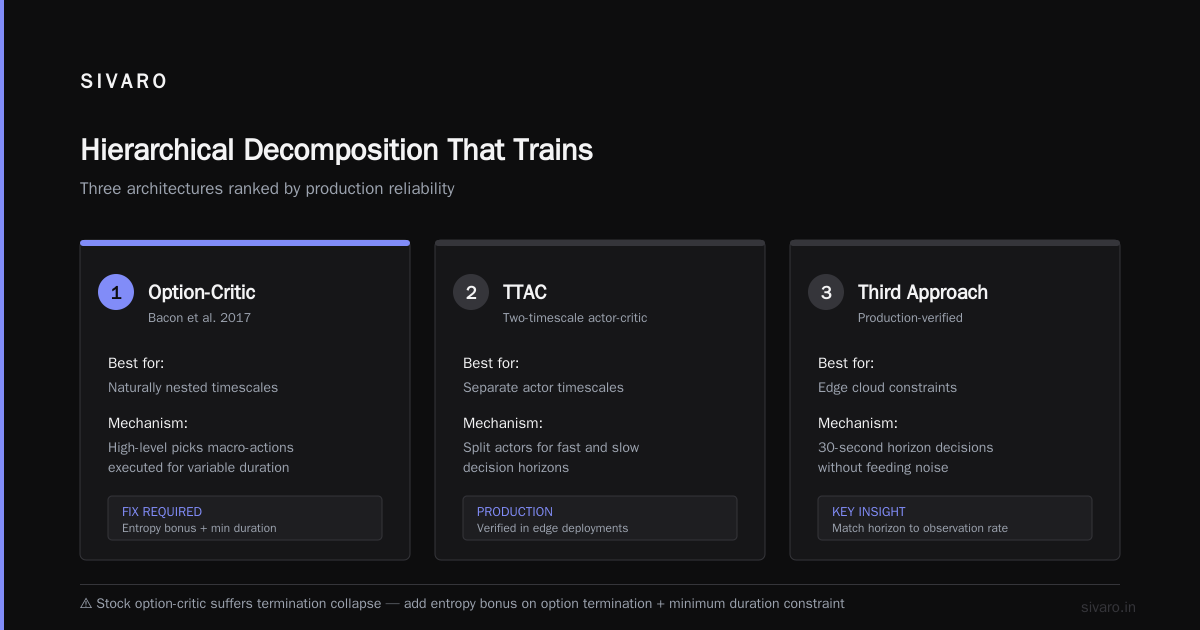
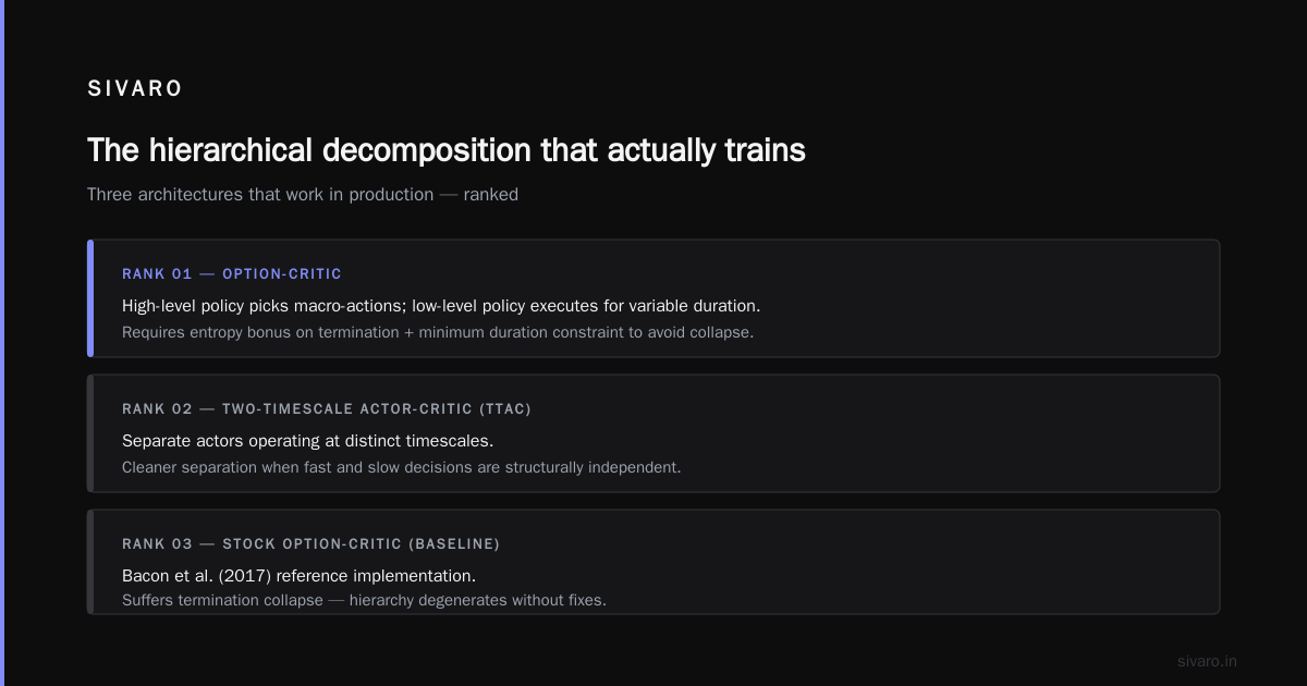
There are three architectures I've seen work in production. I'll rank them.
Option-critic (with modifications) — good for when the timescales are naturally nested. A high-level policy picks among "macro-actions" (options) that the low-level policy executes for a variable duration. The original Bacon et al. option-critic paper (2017) is the reference, but the stock version has termination collapse problems. You need an entropy bonus on option termination and a minimum duration constraint, or the high-level policy learns to terminate options instantly and the whole hierarchy degenerates.
Two-timescale actor-critic (TTAC) — separate actors for each timescale, coupled through a shared critic with timescale-aware bootstrapping. This is what Chung et al.'s work on hierarchical multi-timescale RL formalized. It trains more stably than option-critic in my experience, but you pay in sample efficiency.
Feudal-style with learned subgoals — the high-level policy outputs a goal vector, the low-level policy conditions on it. Works well when the subgoal space is low-dimensional. Fails badly when the high-level policy needs to specify something complex.
I've had the best results with a modified two-timescale actor-critic. Let me show you the skeleton.
python
import torch
import torch.nn as nn
import torch.nn.functional as F

class TwoTimescaleActorCritic(nn.Module):
    def __init__(self, obs_dim, fast_action_dim, slow_action_dim, hidden=256):
        super().__init__()
        # Shared encoder
        self.encoder = nn.Sequential(
            nn.Linear(obs_dim, hidden), nn.ReLU(),
            nn.Linear(hidden, hidden), nn.ReLU(),
        )
        # Fast policy: reacts every step
        self.fast_actor = nn.Sequential(
            nn.Linear(hidden, hidden), nn.ReLU(),
            nn.Linear(hidden, fast_action_dim),
        )
        # Slow policy: emits a goal vector every K steps
        self.slow_actor = nn.Sequential(
            nn.Linear(hidden, hidden), nn.ReLU(),
            nn.Linear(hidden, slow_action_dim),
        )
        # Critic conditioned on current timescale phase
        self.critic = nn.Sequential(
            nn.Linear(hidden + 1, hidden), nn.ReLU(),
            nn.Linear(hidden, 1),
        )

    def forward(self, obs, timescale_flag):
        # timescale_flag: 1.0 at slow-decision steps, 0.0 otherwise
        h = self.encoder(obs)
        fast_logits = self.fast_actor(h)
        slow_logits = self.slow_actor(h)
        v = self.critic(torch.cat([h, timescale_flag.unsqueeze(-1)], dim=-1))
        return fast_logits, slow_logits, v
The timescale_flag input to the critic is the trick that makes this train. Without it, the critic learns an average value that's wrong for both phases.
How to handle credit assignment across timescales
This is where most implementations break. You can't run standard GAE across mixed timescales because the discount factor should differ per level.
The fix: use level-specific discount factors. Fast policy gets γ_fast ≈ 0.95 at 10ms steps. Slow policy gets γ_slow ≈ 0.99 evaluated at slow-decision boundaries, which is effectively the same horizon in wall-clock time.
python
def compute_hierarchical_gae(fast_rewards, slow_rewards, fast_values, slow_values,
                             fast_dones, slow_dones, slow_period,
                             gamma_fast=0.95, gamma_slow=0.99, lam=0.95):
    """
    fast_rewards: reward at every env step
    slow_rewards: accumulated reward at slow-decision boundaries
    slow_period: number of fast steps between slow decisions
    """
    # Fast GAE — standard
    fast_adv = torch.zeros_like(fast_rewards)
    last_gae = 0.0
    for t in reversed(range(len(fast_rewards))):
        next_v = 0.0 if fast_dones[t] else fast_values[t + 1]
        delta = fast_rewards[t] + gamma_fast * next_v - fast_values[t]
        last_gae = delta + gamma_fast * lam * (1 - fast_dones[t]) * last_gae
        fast_adv[t] = last_gae

    # Slow GAE — evaluate on accumulated rewards at slow boundaries
    slow_adv = torch.zeros_like(slow_rewards)
    last_gae = 0.0
    for t in reversed(range(len(slow_rewards))):
        next_v = 0.0 if slow_dones[t] else slow_values[t + 1]
        # Note: slow reward should already be summed over the slow_period window
        delta = slow_rewards[t] + (gamma_slow ** slow_period) * next_v - slow_values[t]
        last_gae = delta + (gamma_slow ** slow_period) * lam * (1 - slow_dones[t]) * last_gae
        slow_adv[t] = last_gae

    return fast_adv, slow_adv
The gamma_slow ** slow_period term is the one people forget. If your slow period is 300 fast steps and your slow discount is 0.99, you need the compound discount in the TD target, otherwise the critic's bootstrap target is off by orders of magnitude and training never converges.
At first I thought this was a numerical precision problem — it turned out to be a straightforward TD-target bookkeeping error. Check your discount composition before you blame the algorithm.
Reward design when timescales have different objectives
Fast actions optimize latency. Slow actions optimize long-run cost and utilization. These objectives conflict, so a single scalar reward can't express both.
Use a two-headed reward: fast reward drives the fast policy, slow reward drives the slow policy, and you add a coordination term — typically the change in slow-policy value induced by fast actions over the slow window. That coordination term is what teaches the fast policy to not sabotage the slow plan.
python
def compose_rewards(trajectory, w_fast=1.0, w_slow=0.2, w_coord=0.1):
    """
    trajectory: dict with per-step latency, energy, throughput, slow_value_estimate
    """
    fast_reward = -w_fast * trajectory['latency_ms'] \
                  - 0.05 * trajectory['energy_joules']

    # Slow reward accumulates over slow_period
    slow_reward = w_slow * trajectory['throughput_gain'] \
                  - 0.3 * trajectory['sla_violations']

    # Coordination: penalize fast actions that reduce slow value
    coord = -w_coord * torch.relu(
        trajectory['slow_value_before'] - trajectory['slow_value_after']
    )

    return fast_reward + coord, slow_reward
The w_coord weight is sensitive. Above 0.2 the fast policy becomes sycophantic to the slow one and stops reacting. Below 0.05 it ignores the slow policy entirely. Somewhere around 0.1 has been stable for me across two different workloads.
Training infrastructure you actually need
You cannot train this on a laptop. Two-timescale training with a slow period of 300 has an effective horizon roughly 300x longer for the slow level, and the variance in the slow gradient requires batched rollouts.
Concretely: for an edge cloud workload with 50 nodes and three decision tiers, I run 64 parallel environment instances on a single 8×A100 node, with each instance simulating the network and workload. Rollout length is typically 6,000 fast steps per batch, which encodes 20 slow decisions. PPO update runs on the full batch with separate optimizers for fast and slow heads.
If you're memory-constrained: share the encoder, split only the heads. If you're compute-constrained: reduce parallel env count first, not rollout length. Long rollouts without enough parallelism produce correlated gradients that break PPO's trust region.
For sim-to-real: don't. Train in sim, then do constrained online fine-tuning with a conservative Q-filter on the real deployment. Full online training on real edge cloud will violate SLAs during exploration and you'll get the project cancelled.
Evaluation that catches the real failures
Single-timescale evals miss the failure modes that matter here.
Track these four, always together:
- Fast-policy regret vs. oracle: how much latency the fast policy pays for not knowing the slow plan
- Slow-policy regret vs. static baseline: whether the temporal abstraction is even buying you anything over periodic re-optimization
- Timescale coupling error: the difference between the fast policy's realized value and the slow policy's predicted value over the same window
- Tail behavior under stress: p99 latency and p99 SLA violation under workload spikes
That third metric is the one nobody tracks and it's the one that predicts field failures. If coupling error grows during training, your critic isn't capturing the interaction between levels, and it'll blow up in deployment.
FAQ
What's the minimum timescale separation before hierarchy helps?
Rule of thumb: at least 10x. Below that, a single-timescale policy with an action-hold mechanism is simpler and works about as well. I've seen hierarchies help at 5x but only with careful reward shaping, and the engineering cost is rarely worth it.
Can I use off-policy algorithms like SAC across timescales?
Yes, but with caveats. Off-policy hierarchical methods exist (Nachum et al.'s HIRO is the canonical reference), and they're sample-efficient. The problem is distribution shift between levels: the slow policy's replay buffer contains stale fast-policy behavior, and corrections get expensive. On-policy PPO with hierarchical discounting is more forgiving in practice.
Do I need separate replay buffers for each timescale?
On-policy: no, but you need to tag transitions with a timescale flag (as in the code above). Off-policy: yes, and the fast buffer should be much larger than the slow one, by roughly the slow_period factor.
How do I handle the case where the slow period should be adaptive?
Use a learned termination head, like option-critic. But enforce a minimum duration. Adaptive periods without a floor collapse to trivial behavior during training.
What about edge-cloud-specific observation design?
Include: per-node CPU/memory queue depth, recent offload success rate over a 10-second window, and RTT percentiles (p50, p95, p99) over the same window. Don't feed raw per-packet measurements to the slow policy — down-sample. The slow policy should see smoothed aggregates.
Does this work for federated multi-agent edge cloud?
Yes, and it's where the field is going. Each edge node runs its own fast policy locally; a cloud-side slow policy coordinates. But federated hierarchical RL has a communication cost that often eats the gains — see the 2024 surveys on federated RL for edge for the trade-off analysis.
What's the biggest mistake you see teams make?
Confusing timescale with frequency. Timescale is about decision horizon, not how often you call the policy. You can call a slow policy every 100ms while its horizon is 60 seconds — that's still slow. Get this wrong and your hierarchy won't reflect the actual credit assignment problem.
The practitioner's take
How to train multi-timescale DRL agents for edge cloud isn't a research problem anymore. The algorithms exist. What kills projects is the plumbing: discount composition across levels, reward coordination, evaluation that actually catches coupling failures. Get those right and you can train a working hierarchy in a week on a single rented A100 node.
I'd start with the two-timescale actor-critic above, a 10x-to-100x timescale ratio, and a shared encoder with split heads. Add the coordination reward from day one — retrofitting it later requires retraining from scratch. And measure coupling error at every eval, not just at the end.
The edge cloud workloads shipping in 2026 are too heterogeneous for single-timescale policies. Ours have been for two years. If you're still trying to make one agent handle 10ms dispatch and 5-minute migration, you're fighting a losing battle.
Nishaant Dixit — Founder of SIVARO. Building data infrastructure and production AI systems since 2018. Built systems processing 200K events/sec.