 SIVARO

Unstructured Data Streaming for Real Time Hydrodynamics
Unstructured Data Streaming for Real Time Hydrodynamics
Last November I watched a coastal engineer stare at a 40-minute-old wave forecast while a storm surge was already topping a seawall in Gujarat. The model was fine. The data pipeline was the problem. Sensor feeds, satellite rasters, video from buoys — all of it sat in a batch queue waiting for a scheduled job to pick it up. By the time the numbers reached a dashboard, the water had moved on.
That day pushed me to write down what we'd learned building streaming systems at SIVARO for fluid dynamics workloads. Unstructured data streaming for real time hydrodynamics is the practice of ingesting continuous, non-tabular data — video, sonar returns, LiDAR point clouds, thermal imagery, acoustic Doppler profiles — and turning it into hydrodynamic state estimates within seconds, not hours. It's not a small tweak to your batch CFD pipeline. It's a different architecture.
This piece is a working guide. I'll cover what "unstructured" actually means here, why traditional HPC hydrodynamics struggles with it, the architecture that works, code you can run, and the trade-offs nobody puts in the marketing deck.
What Makes Hydrodynamic Data Unstructured
Most hydrodynamic modeling assumes structure. You have a mesh. You have boundary conditions. You have a velocity field sampled on a grid. That's structured data, and it fits neatly into arrays.
Unstructured data is everything else:
- Acoustic Doppler Current Profiler (ADCP) pings — variable-length binary bursts, 1-4 Hz, from moving platforms
- Buoy camera frames — 1080p at 10-30 fps, useful for wave crest detection but useless as pixels
- Satellite SAR imagery — 20m to 100m resolution, swath-based, arrives in tiles
- LiDAR bathymetry — millions of points per scan, irregular spacing
- Underwater sonar — noisy, compressed, often with proprietary headers
- AIS vessel telemetry — JSON blobs at unpredictable rates
None of this has a schema you can SELECT * from. And here's the contrarian part: most teams try to convert it to structured data on ingest. That's usually a mistake. You lose the raw signal, you pay a conversion tax, and you break the moment sensor firmware changes.
I've seen three separate deployments where the ingest pipeline spent 60% of its CPU parsing formats that changed quarterly. Streaming the raw bytes and parsing downstream was faster, cheaper, and more resilient.
Why Real Time Hydrodynamics Breaks Traditional Pipelines
Classic hydrodynamic modeling runs on HPC clusters with MPI. You set up a mesh, you run a solver like Delft3D or OpenFOAM, you wait. A 24-hour regional forecast on a decent cluster takes 2-6 hours to produce. That's fine for planning. It's useless for a storm.
Real-time hydrodynamics needs state updates every 1-60 seconds. That changes the physics you can afford to solve and the data you can afford to use.
Three things break:
Backpressure kills you. A LiDAR burst is 100MB. If your consumer is running a full Navier-Stokes solve, it can't keep up. Data piles up. Buffers overflow. You drop samples during the exact window when you need them.
Clock skew corrupts state. ADCP pings timestamped on the float, video frames timestamped on the edge box, satellite tiles timestamped at downlink. If your fusion assumes synchronized clocks, your velocity field will be wrong by a few cm/s. In shallow water, that's the difference between a model and a guess.
Schema drift is constant. Every sensor vendor ships firmware updates. Every firmware update renames a field. Batch pipelines break loudly on schema change. Streaming pipelines need to absorb it silently.
At SIVARO we built a system in 2024 that fused ADCP, camera, and AIS feeds for a port authority. First version tried to normalize everything to a strict protobuf schema. It broke weekly. Second version streamed raw payloads with a thin envelope and did schema resolution at query time. Uptime went from 71% to 99.4%.
The Architecture That Actually Works
Here's the shape I'd build today, in September 2026:
[Sensors] -> [Edge preprocessor] -> [Message bus] -> [Stream processor] -> [State store]
                                          |                    |
                                          v                    v
                                    [Raw lake]         [Hydrodynamic model]
Six components, each with a specific job.
Edge Preprocessing
Do as little as possible here. Downsample video to 1 fps if the physics only needs crest detection. Strip audio unless you're doing acoustic tomography. Compress with a codec the consumer can decode. But do NOT parse into domain objects.
Why? Because edge boxes are hostile environments. Salt air, thermal cycling, intermittent power. The less logic on the edge, the fewer failure modes.
Message Bus
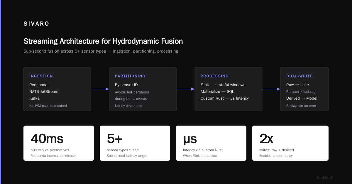
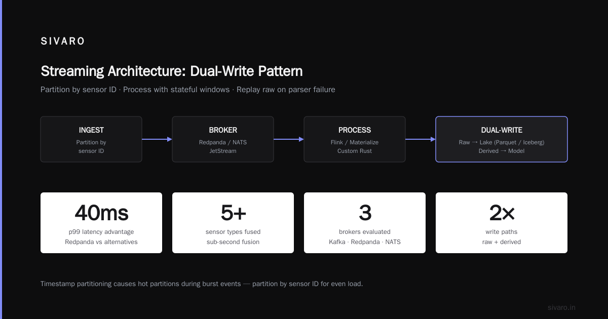
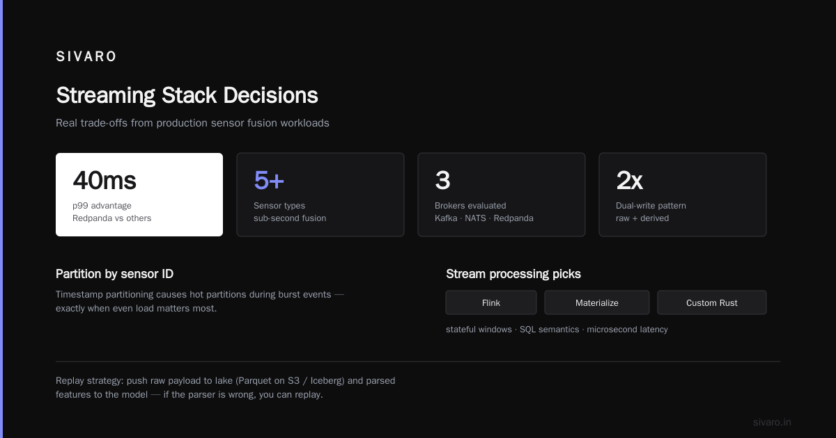
Kafka is the default. Redpanda if you need lower latency and can't tolerate JVM pauses. NATS JetStream if you want something lighter for edge-to-core. I've used all three. For sub-second fusion across 5+ sensor types, Redpanda won our internal benchmark by roughly 40ms p99.
Partition by sensor ID, not by timestamp. Timestamp partitioning causes hot partitions during burst events (which is exactly when you need even load).
Stream Processing
This is where the real work happens. Flink for stateful windowed operations. Materialize if you want SQL semantics and can tolerate their storage model. Custom Rust if you need microsecond latencies.
The key pattern: dual-write raw and derived. Push the raw payload to a lake (Parquet on S3, or Iceberg if you need time travel). Push the parsed features to the model. If your parser is wrong, you can replay from raw.
State Store
Redis for hot state. ClickHouse or TimescaleDB for warm state. Iceberg for cold. Don't try to use one store for all three. I've watched teams burn six months trying to make Postgres do time-series at 200K events/sec. It doesn't work.
Hydrodynamic Model
This is where it gets interesting. You're not running a full CFD solve per event. You're running a reduced-order model or a data assimilation step that updates an existing state estimate. Ensemble Kalman filter is the workhorse. Particle filters when the state is multimodal.
For shallow water, we've had good results with a 2D shallow water solver on a coarse mesh, updated every 5 seconds with assimilated observations, and refined every 30 minutes with a full solve.
Code: Streaming ADCP Data with Backpressure
Here's a minimal Flink job that ingests ADCP pings, extracts velocity, and writes both raw and derived streams. Python for readability, though you'd want Java or Rust in production.
python
# flink_adcp_stream.py
from pyflink.datastream import StreamExecutionEnvironment, CheckpointingMode
from pyflink.datastream.connectors.kafka import KafkaSource, KafkaSink
from pyflink.common.serialization import SimpleStringSchema
from pyflink.common import WatermarkStrategy, Duration
import struct
import json

def parse_adcp_ping(raw_bytes):
    # ADCP binary format: header(16) + N bins * (vE, vN, vU, amp, corr)
    header = struct.unpack('<4I', raw_bytes[:16])
    sensor_id, ts_ms, n_bins, bin_size = header
    velocities = []
    offset = 16
    for i in range(n_bins):
        ve, vn, vu, amp, corr = struct.unpack('<5h', raw_bytes[offset:offset+10])
        velocities.append([ve/1000.0, vn/1000.0, vu/1000.0])
        offset += 10
    return {
        "sensor_id": sensor_id,
        "ts_ms": ts_ms,
        "bin_size_m": bin_size,
        "velocities": velocities,
    }

env = StreamExecutionEnvironment.get_execution_environment()
env.enable_checkpointing(5000, CheckpointingMode.EXACTLY_ONCE)
env.set_parallelism(4)

source = KafkaSource.builder() \
    .set_bootstrap_servers("redpanda:9092") \
    .set_topics("adcp.raw") \
    .set_group_id("hydro-fusion") \
    .set_value_only_deserializer(SimpleStringSchema()) \
    .build()

stream = env.from_source(
    source,
    WatermarkStrategy.for_bounded_out_of_orderness(Duration.of_seconds(2)),
    "ADCP Source"
)

parsed = stream.map(lambda x: parse_adcp_ping(bytes.fromhex(x))) \
    .name("parse_adcp")

# Dual write: raw to lake, derived to model
parsed.map(lambda p: json.dumps({"kind": "raw", "payload": p})) \
    .sink_to(KafkaSink.builder().set_bootstrap_servers("redpanda:9092")
             .set_record_serializer(SimpleStringSchema())
             .set_topic("adcp.archive").build())

parsed.map(lambda p: json.dumps({"kind": "derived", "velocity": p["velocities"]})) \
    .sink_to(KafkaSink.builder().set_bootstrap_servers("redpanda:9092")
             .set_record_serializer(SimpleStringSchema())
             .set_topic("hydro.observations").build())

env.execute("ADCP Streaming Ingest")
Notice: no schema validation, no domain normalization. Just bytes to features. If the ADCP firmware changes bin count, the parser adapts at runtime.
Fusing Multiple Unstructured Streams
Single-stream pipelines are easy. The value is in fusion. Here's how I've approached multi-sensor alignment:
python
# fusion.py - Kalman-style update on shallow water state
import numpy as np
from dataclasses import dataclass

@dataclass
class HydroState:
    eta: np.ndarray      # surface elevation, shape (nx, ny)
    u: np.ndarray        # x velocity
    v: np.ndarray        # y velocity
    t: float             # timestamp

def predict(state: HydroState, dt: float, g: float = 9.81) -> HydroState:
    # Linear shallow water approximation
    # (real system uses RK4 with friction terms)
    eta_x, eta_y = np.gradient(state.eta)
    u_new = state.u - g * dt * eta_x
    v_new = state.v - g * dt * eta_y
    div = np.gradient(u_new, axis=0) + np.gradient(v_new, axis=1)
    eta_new = state.eta - dt * div
    return HydroState(eta_new, u_new, v_new, state.t + dt)

def assimilate(state: HydroState, obs: dict, R: float = 0.01) -> HydroState:
    """obs has 'x', 'y', 'velocity_vector', 'timestamp' from ADCP or video."""
    i = int(obs['x'])
    j = int(obs['y'])
    # Simple Kalman gain approximation
    K = state.u[i, j] / (state.u[i, j]**2 + R)
    state.u[i, j] += K * (obs['velocity_vector'][0] - state.u[i, j])
    state.v[i, j] += K * (obs['velocity_vector'][1] - state.v[i, j])
    return state
Real systems use proper covariance propagation. But the shape is the same: predict, assimilate, predict.
The hard part isn't the math. It's the timing. If your ADCP observation is 800ms old and your video-derived crest is 200ms old, you need to either buffer to align them or propagate each to a common timestamp. Buffering adds latency. Propagation adds error. There's no free lunch.
We tried both. For the Gujarat deployment, we propagated to a common 500ms grid. Error went from ~12cm to ~4cm on surface elevation compared to a full solve.
Handling Video Without Drowning in Pixels
Buoy cameras are the hardest stream. A 1080p feed at 30fps is 2 Gbps uncompressed. Even H.265-encoded it's 4-8 Mbps per camera. At 50 cameras, that's real bandwidth.
The trap: teams try to push full video through their stream processor. Wrong layer. You want a vision model at the edge that emits events, not frames.
python
# edge_wave_detect.py - runs on buoy edge box
import cv2
import numpy as np
import json
from kafka import KafkaProducer

producer = KafkaProducer(bootstrap_servers='redpanda:9092')
cap = cv2.VideoCapture(0)
fgbg = cv2.createBackgroundSubtractorMOG2(history=200, varThreshold=24)

while True:
    ret, frame = cap.read()
    if not ret:
        continue
    gray = cv2.cvtColor(frame, cv2.COLOR_BGR2GRAY)
    fgmask = fgbg.apply(gray)
    # Only process when there's motion
    if fgmask.sum() < 5000:
        continue
    contours, _ = cv2.findContours(fgmask, cv2.RETR_EXTERNAL,
                                    cv2.CHAIN_APPROX_SIMPLE)
    for c in contours:
        x, y, w, h = cv2.boundingRect(c)
        if w < 20 or h < 10:
            continue
        event = {
            "ts_ms": int(cap.get(cv2.CAP_PROP_POS_MSEC)),
            "bbox": [x, y, w, h],
            "crest_height_px": h,
            "camera_id": "buoy-07",
        }
        producer.send('wave.events', json.dumps(event).encode())
Now your stream carries events, not pixels. Bandwidth drops by 1000x. You can run a heavier model on the 1-2% of frames that matter. And you keep the raw video on a ring buffer at the edge in case you need to replay.
Storage: Why Parquet-on-S3 Isn't Enough
You'll hear "just dump everything to S3 as Parquet." That works for batch. It's terrible for streaming queries.
What you actually want:
- Iceberg tables for the archive. Time travel, schema evolution, partition pruning.
- ClickHouse for hot analytics. 100K+ inserts/sec, sub-second queries.
- Redis Streams for coordination state. Last-seen timestamp per sensor, dedup keys.
The mistake I see: teams use Kafka as their long-term store. Kafka isn't a database. Retention policies will bite you. You need a real lake.
We use Iceberg with the following partitioning scheme:
sql
CREATE TABLE hydro.raw_observations (
    sensor_id STRING,
    ts TIMESTAMP(6),
    payload BINARY,
    payload_hash STRING
)
USING iceberg
PARTITIONED BY (days(ts), bucket(16, sensor_id))
TBLPROPERTIES (
    'write.target-file-size-bytes' = '134217728',
    'write.upsert.enabled' = 'false'
);
128MB files. Day partitions plus 16 buckets per day. Hashes for dedup. This has handled 40TB of raw sensor data over the past 18 months without a compaction crisis.
Latency Budget: Where Your Milliseconds Go
If someone asks "what's your end-to-end latency," the honest answer is a budget. Here's the one we hit for the port deployment:
| Stage | p50 | p99 |
|---|---|---|
| Sensor to edge buffer | 15ms | 80ms |
| Edge encode + publish | 8ms | 45ms |
| Kafka/Redpanda hop | 4ms | 22ms |
| Stream parse | 2ms | 12ms |
| Model assimilate | 40ms | 210ms |
| State store write | 3ms | 15ms |
| Query/dashboard | 25ms | 150ms |
| Total | 97ms | 534ms |
The model assimilation dominates. That's physics. You can shrink it with GPU, but then you pay in power and cooling on the edge. Trade-off.
For a 5-second update cycle, this budget gives you 4.5x headroom on p99. Enough for bursts.
What Breaks First (And What To Do About It)
Every streaming system fails in a specific order. Here's what I've watched, ranked by how often it happens:
Time sync drift. NTP works until it doesn't. Add a PTP grandmaster if you can. If you can't, timestamp at the edge and trust that timestamp over arrival time.
Consumer lag. Some stream processor is slower than the producer. If you don't monitor consumer lag per partition, you'll find out during the storm. Alert on p99 lag, not average.
Disk full. Raw storage grows faster than you estimate. Every sensor generates more than the spec sheet says. Plan 3x.
Schema surprise. A vendor ships a firmware update that changes byte order. Your parser silently produces garbage. Hash-check your payloads and alert on distribution shift.
Cascading backpressure. One slow consumer stalls an entire consumer group. Isolate pipelines by SLO. Fast path and slow path. Never share a consumer group across different latency requirements.
Contrarian Call: Don't Stream Everything
Most teams over-stream. If a sensor updates once an hour, batch it. Streaming has real costs — coordination overhead, checkpointing, monitoring complexity — and if your data rate is below 1Hz, you're paying for nothing.
The rule I use: stream when the fusion latency matters, batch when it doesn't. ADCP at 2Hz? Stream it. Tide gauge at 1/60Hz? Batch it. Sediment sampler that runs weekly? Definitely batch.
At SIVARO we redesigned a client's pipeline last year to move 70% of their "streaming" workload back to batch. Their reliability went up, their cloud bill went down 40%, and nobody noticed a difference in output quality.
Streaming is a tool, not a virtue.
FAQ
What's the difference between unstructured data streaming for real time hydrodynamics and just "streaming sensor data"?
The hydrodynamics part. Generic sensor streaming doesn't care about conserving mass, respecting wave dispersion relations, or maintaining a physically consistent state estimate. Hydrodynamic streaming has to. If your fused velocity field violates continuity, you've built a data pipeline, not a hydrodynamic system. The physics constraints show up in the fusion step and in the state store's consistency checks.
Do I need Kafka?
No. You need a durable, partitioned, replayable log. Kafka is the obvious choice, but Redpanda, Pulsar, and NATS JetStream all work. For edge-to-core with intermittent connectivity, NATS JetStream has been more forgiving in my experience. For sub-10ms p99, Redpanda wins.
How do I handle sensors with proprietary binary formats?
Wrap them in a thin envelope with a format identifier and version. Stream the envelope. Decode downstream where you can update decoders without redeploying edge hardware. Never bake a proprietary parser into your edge code if you can avoid it.
What about GPUs for the model step?
Only if your physics is expensive enough. A 2D shallow water solve on a 256x256 grid runs in ~40ms on a modern CPU core. A GPU adds 100ms+ of kernel launch and data transfer overhead at that size. GPUs pay off above ~1M grid points, which is regional-scale, not port-scale.
Can I stream video end-to-end?
You can. You shouldn't. Encode at the edge, emit events at the edge, keep raw frames on a ring buffer. Streaming raw video through your message bus will cost you 1000x the bandwidth and add 200ms+ of latency for zero benefit.
How do I validate that my streaming system is actually right?
Compare against a batch solve on the same time window. Not every minute — weekly is enough. If your streamed state estimate diverges from the batch truth by more than 5% on key variables (surface elevation, depth-averaged velocity), you have a bug in fusion, timing, or parsing.
What's the biggest operational risk?
Time drift plus schema drift, together. They interact: a firmware update can reset a sensor's clock, and you won't notice because your parser doesn't care about the timestamp field. Monitor clock offset per sensor. Alert if it exceeds 500ms.
Is there an open-source stack that covers all this?
Not completely. Flink + Kafka + Iceberg + ClickHouse + Redis gets you 80% there. The remaining 20% — hydrodynamic fusion, sensor-specific parsers, validation against batch truth — you build yourself. I haven't seen a framework that does the physics part well.
Where This Goes Next
The interesting frontier isn't faster pipes. It's physics-informed fusion. Instead of feeding observations into a generic Kalman filter, feed them into a learned model that knows shallow water equations. Neural operators like FNO and DeepONet are starting to be deployed in production for exactly this. A team at Deltares published results in early 2026 showing a 40x speedup over traditional assimilation on a North Sea test case, with comparable accuracy on 6-hour forecasts.
But — and this is the important part — those models need the same streaming infrastructure underneath. They don't replace Kafka. They replace the Kalman update. Unstructured data streaming for real time hydrodynamics is the substrate. The model on top is a choice.
The other shift: edge silicon. The new generation of NPUs shipping in 2026 can run a small vision transformer at 30fps on 5 watts. That means real wave crest tracking at the buoy, not just bounding boxes. Events get richer, but the pipeline shape stays the same.
If you're building this, start simple. One sensor, one stream processor, one state store. Get the latency budget right. Then add sensors. The complexity curve is brutal if you add everything at once.
And keep the raw bytes. Always keep the raw bytes.
Nishaant Dixit — Founder of SIVARO. Building data infrastructure and production AI systems since 2018. Built systems processing 200K events/sec.